
Geographic Profiling technique is used to find the origin of a series of crimes. The method was recently extended to other fields. One of the best renowned data in epidemiology is that by John Snow during an outburst of cholera in London. We wrote Python scripts to perform the analyses to apply the Geographic Profiling for individuating the starting origin of an infection by using the old Snow's data set. We modified the method by applying a weight to each point of the map where cases of cholera were reported. The weight was proportional to the number of cases in a given location.
This modification of the Geographic Profiling method allowed to individuate in the map an area of maximum probability of the infection source, which was a few meters wide and including the historically known source of cholera, that is the “classical” water pump at Broad Street.
The method appears to be a useful complement in order to individuate the source of epidemics when available data about the cases of the infections can be summarized on a map.
Geographic Profiling (GP) is an analytic tool widely used in criminology in order to identify on a map an area of highest probability assumed to contain the origin of linked events, typically crimes executed by a serial offender.1 The method was extended from criminology to other fields where it was possible to identify a series of linked events which might have originated from a starting point in the space (represented on a two dimensional map). Fields of application other than criminology have been: invasion by alien species,2–5 bumblebees foraging and nest location,6,7 and infectious diseases targeting.8,9
GP uses the coordinates on the mapped events, creating a probability surface, the so-called geoprofile.1 The geoprofile does not indicate the exact origin of the events, but rather prioritize a series of geographical points, based on the data.1 The geoprofile will provide on the map a decreasing probability density of finding the source of the events drawn on the map.1
The model does not search simply the geographical center of the events, but instead it considers a distance-decay function, such that the probability of an event will be lower by increasing the distance from the center of origin; and a buffer zone, within which the probability of an event tends to zero.1 The distance-decay function is related to maximizing parsimony in movement, in economical and energy terms. Surprisingly, these functions revealed to be found not only for humans (criminals), but also even for invasive (not human) species2,3 and infectious diseases.8–10
The need for analytical tools to recognize the source of the spreading of “something” (generally a threat) has always been an important task.11 One of the best known cases is, in epidemiology, that of cholera outbreak in London, 1854, studied by John Snow12 and widely cited as a seminal work in spatial epidemiology13 [13 and references therein]. Dr. Snow tagged the cholera cases and the water pumps on the map of London and searched for the area with the highest number of cases, so discovering that the origin of the outbreak (the so-called focus of infection) was a contaminated water pump in Broad Street. The tagged cholera cases drawn by Snow on the map of London can be converted in a data set of coordinates, that was already used by Le Comber et al.8 to test the GP method for targeting infectious diseases. Le Comber et al.8 were able to mark a restricted area in the map of London containing the famous water pump of Broad Street (see Fig. 1C and D in their article). These authors used as input data the individual addresses where case of deaths due to cholera had occurred, that is 321 addresses, while the total number of cases amounted to 575, since more than one case might have occurred at the same address. Le Comber et al.8 used this approach “to avoid the possible problem of spatial temporal non-independence due to secondary infections at a given address”. Our approach included, instead, all cases assigning a weight to each point (addresses) proportional to the number of cases. We overlooked possible secondary human-to-human contagions, since cholera should not easily transmit from person-to-person, while its transmission is known to be more food- or water-born.14 For this reason, we interpreted more than one case in the same address as independent events and hence summable.
Therefore, here we propose a new method of applying GP in which a different weight is assigned to each point of the map proportionally to the number of cases occurred in each point.
MethodsThe data about the positions of cases on the map were acquired with Neuronmorpho (http://www.southampton.ac.uk/∼dales/morpho/), a plugin of ImageJ (National Institute of Health; http://rsb.info.nih.gov/ij/), that can read a map position with a mouse click, building a csv file containing the coordinates point by point. Weights were added manually. Our method calculates the GP by weighting each point of the map in direct proportionality with the number of cases occurred in a given point of the map. That is, some points of the map are more important than others. The data were analyzed with a Python script (Geoprof3.0.2.py).
Crucial for the GP analysis is the assignment of the values B, corresponding to the radius of the buffer zone.2 In our analysis we used B=30, corresponding to a buffer zone of 30 pixels (about 15m on our map), that is quite small, with respect to other GP analyses in other fields, such as those on malaria cases in Cairo.9 We evaluated more B values, calculating the impact on the analysis. The GP technique is described in detail in Papini et al.3 The variable B (the buffer zone) is of course dependent on the map magnification and on the map resolution, since B is expressed in pixels, while the actual meaning of the buffer zone can be understood only if expressed in meters or km.
The Python scripts were written by the authors and can be retrieved from the site www.unifi.it/caryologia/PapiniPrograms.html. The scripts were executed with Python 2.7.3 (http://www.python.org/), running in Ubuntu 12.04 LTS operating system, kernel 2.6.32. The Python (>=2.6 version) programs need NumPy (http://www.numpy.org/), SciPy (http://www.scipy.org/), Matplotlib (http://matplotlib.org/), Scikit-learn (http://scikit-learn.org), and Python Image Library – PIL – (http://www.pythonware.com/products/pil/) libraries installed. A note about the software is provided as Supplementary material (SoftwareUsesupplementary.pdf).
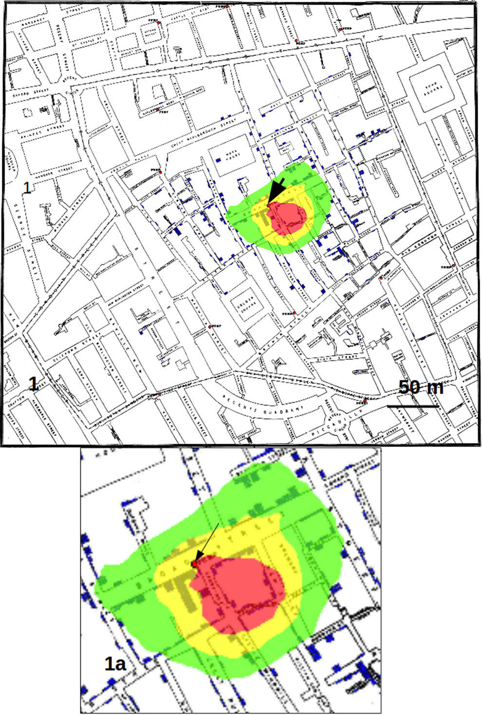
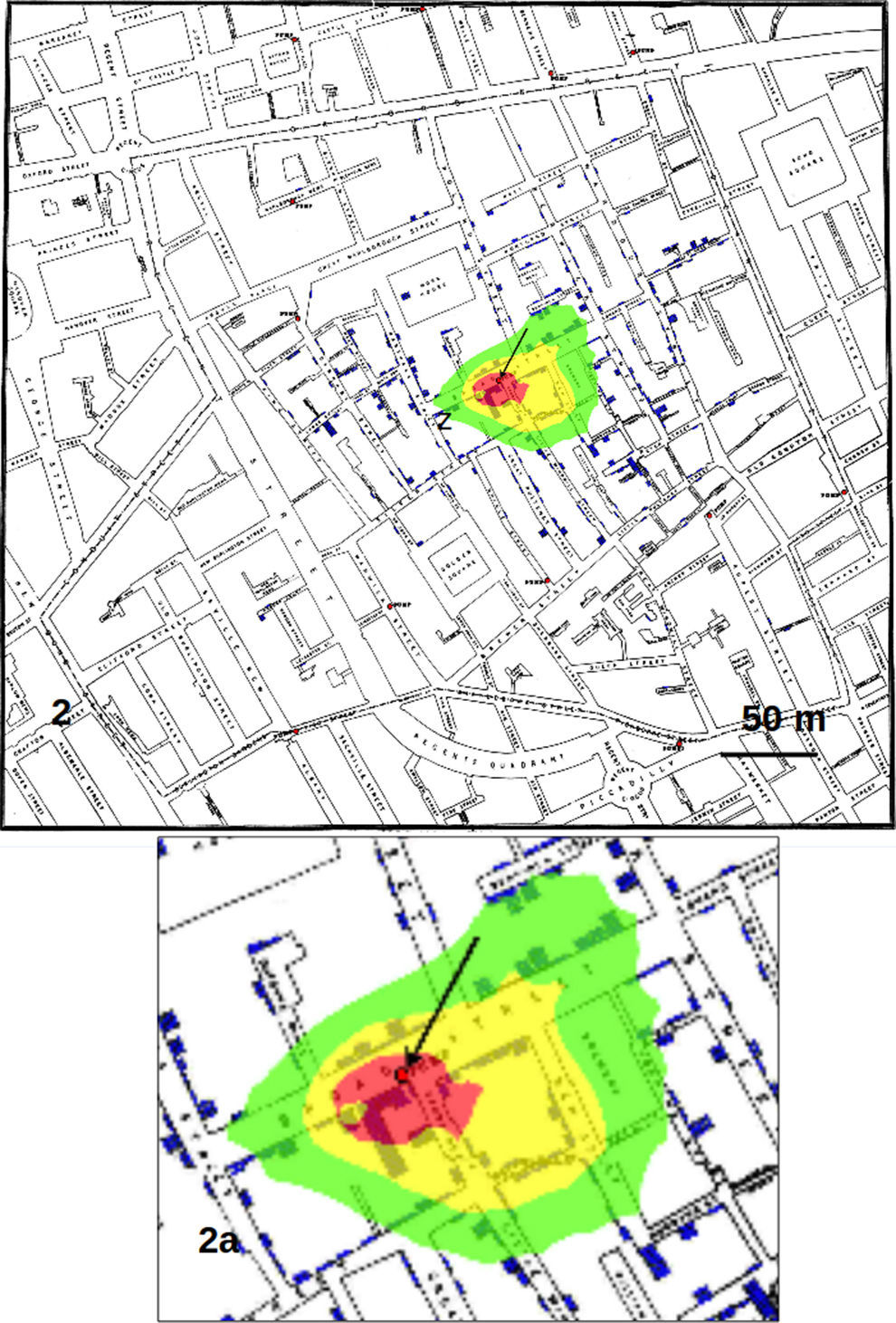
Results and discussionFig. 1 shows the results obtained by considering only the addresses on the map as data sets, corresponding to the analysis by Le Comber et al.,9 that is, no weight was assigned to an address on the basis of the number of recorded cases. In Fig. 2 we show the GP analysis with weights assigned to each point of the map on the basis of the number of cases. The result is quite striking, since the red area, representing the area of the map with the points with 95% of highest probability comprised the pump of Broad Street. This area was about 30m in diameter. With respect to the method that does not consider the number of cases as weights (shown in Fig. 1), the total area of highest probability of the presence of the source was hence much smaller.

 is only about 30m in diameter and it comprises the famous pump of Broad Street.")
Counting the pixels with highest probability of finding the source of the crimes, we found that the red pixels (those with highest probability) decreased substantially passing from considering only the addresses to using the whole data set with weights, that is from 36533 to 10068 (visible from the reduction in dimension of the red area from Fig. 1 to Fig. 2). Calculating each case as a single point, also if located in the same position on the map (that is at the same address), produced an area of red pixels only slightly higher with respect to the use of weights (data not shown).
Calculating the distance on the map, the GP analysis with weights produced an area of maximum probability of finding the source of about 30m in diameter, which contains the well known source of cholera cases in London, that is the famous pump of Broad Street recognized by Snow.12 This result shows that the use of weights proportional to the number of cases in each address largely increase the precision of the analysis, that is, it reduces the area of maximum probability where to look for the source with respect to other GP techniques as those employed by Le Comber et al.9 and Verity et al.11
ConclusionThe weighted geoprofiling can be a useful method to identify a center of origin of an outbreak of a disease, in cases when more cases of infection can be found in the same point of the map (normally corresponding to a residence), largely reducing the priority points and hence showing the highest precision in delimiting the source search area.
The use of weights for more cases of infections at the same address, can be a good choice only in cases where secondary person-to-person infections can be considered not probable (as it is likely the case of cholera), otherwise, as stated by Le Comber et al.9 it is necessary to use as input data each address (point on the map) as points with the same weight=1.
FundingFinancial support by the Italian Ministry of Research (MUR), Fondi di Ateneo.
Conflicts of interestThe authors declare no conflicts of interest.
The following are the supplementary data to this article:
